on
ComputerScience DataScience
arXiv Paper Authors Relation Graph
On 28 December 2021, I downloaded this arXiv AI paper dataset from Kaggle to play around with during the vacation. I ended up exploring it until early in January 2022. The following image is a screenshot of the dataset when displayed on JupyterLab.
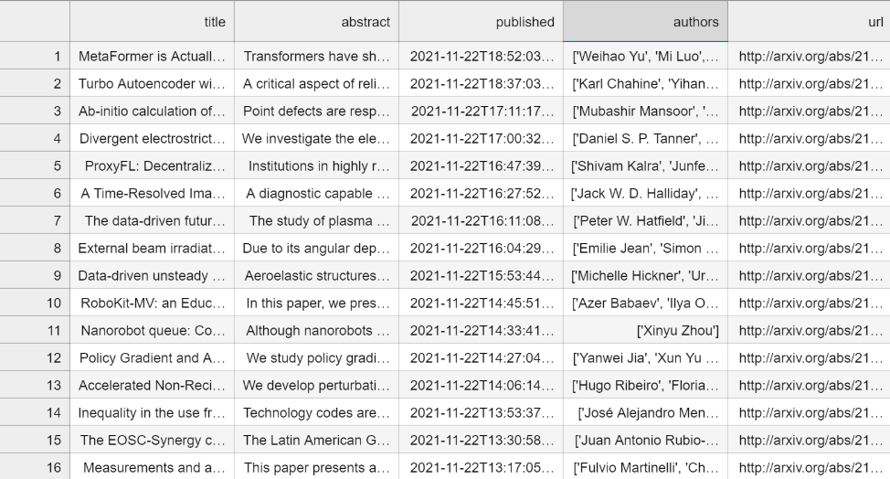
Inspecting the Dataset
We can see in the authors column, the list of authors are kept as valid string representations of Python lists. From here, I decided to focus on the authors column to try building a network of coauthors.
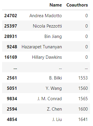
There are people who have a seemingly abnormally high number of coauthors in the dataset, given that there are only 8,000 paper entries in the dataset I retrieved from Kaggle and the dataset only contains AI papers published starting from 2021-07-07 to 2021-11-22.
The following is the summary of the distribution of the number of coauthors an author has during the period.
| count | 37603.000000 |
| mean | 75.658112 |
| std | 225.142775 |
| min | 0.000000 |
| 25% | 3.000000 |
| 50% | 6.000000 |
| 75% | 19.000000 |
| max | 1641.000000 |
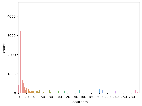
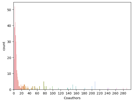
The following is a chart showing the distribution which we take only up to 300 coauthors for better visualization on the area of the first three quartiles.
Problem Definition
Looking at the data, there is a possibility where people with abnormally large number of coauthors are actually multiple people who’re identified by the same identifier in the dataset. Given that people are identified either using their full names or the abbreviated version of their full names, it’s reasonable to think that multiple people with the same name identifier could appear in the dataset.
We’d like to try looking at the data to see if we can predict whether an author entry in the data is really just one person, or it is a combined entry of multiple people with the same name.
In order to do that with only the list of coauthors that have collaborated with the author which we want to determine whether their entry is really an entry of one person or multiple people identified as one, we might be able to try analyzing the relational graph between their registered coauthors.
The following is the visualization of the relation between the coauthors of the first 8 authors in the adjacency list built as the representation of the coauthorship relational graph using NetworkX.
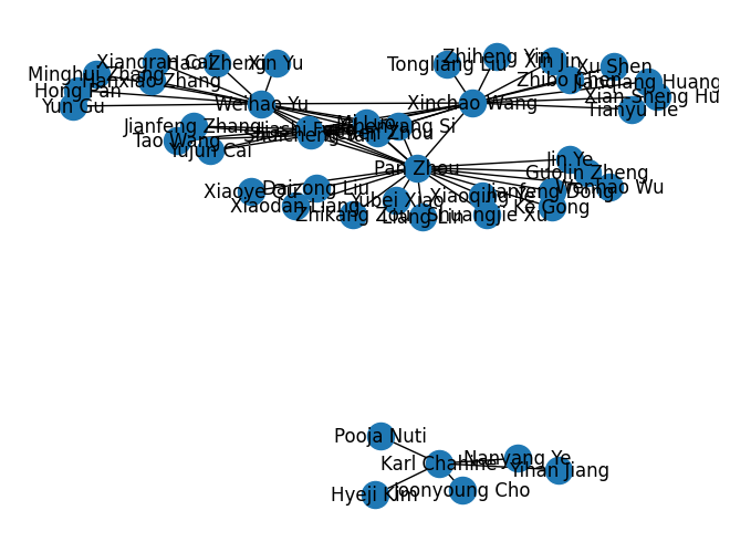
We can see that clusters are formed by the vertices connected to each other. In the following graph, we can see the clusters formed by coauthors of Jin Ye and Weihao Yu.
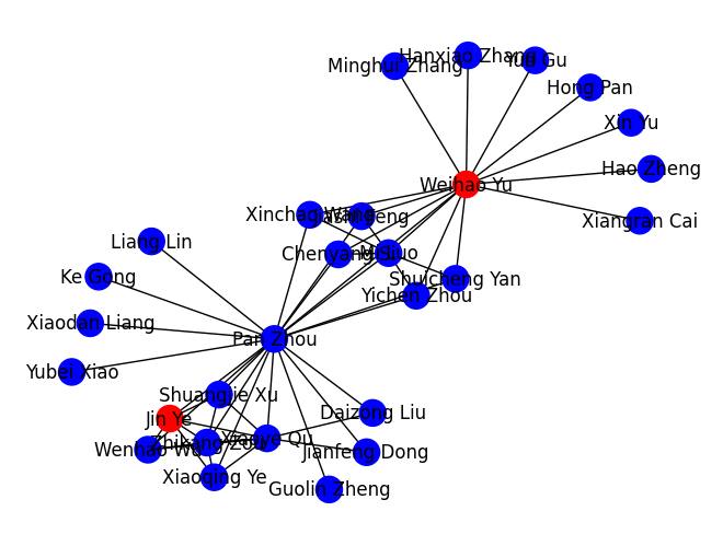
We performed a tree search with depth 2 with Jin Ye and Weihao Yu as the root nodes, then built the graph in the image above. Visually, we can see a distinction of the set of people working with Jin Ye and people working with Weihao Yu. But if by any chance, both Jin Ye and Weihao Yu’s vertices were merged into one joint vertex, could we identify the vertex as connected to the network of two (or possibly even more) distinct researchers?
In this case, our interest is to check with an experiment to see whether it’s possible for us to determine whether a vertex belongs to only one researcher or to multiple researchers.
Our hypothesis is that there’s a difference in the pattern of how the coauthor vertices are connected to each other in the case of where an author’s vertex is a representation of only one person if compared to the case where an author’s vertex is actually a representation of multiple different people.
To formalize it, suppose we have graph \(G\) containing the vertices \(v \in V\) where \(V\) is a set of all author identifiers in the dataset. For each \(v'_d \in V'_d\) where \(V'_d\) is the set of vertices in graph \(G\) which is connected to \(v\) to the degree of \(d\), where the degree \(d\) is the number of hops it takes for \(v\) to reach \(v'_d\).
In the case where we have an author \(a\) where \(a \in V\) and coauthors \(C \subset V\) which are the first degree neighbors of \(a\), where \(C = N(a)\) and \(N(a)\) is the set of first degree neighbors of \(a\). For each \(c \in C\) we’re going to calculate the how many members of \(C\) are also direct neighbors with \(c\) to measure the similarity of \(c\) with \(a\) as follows.
\[S(a, c, d) = \frac{\vert I_{a, c, d} \vert}{\vert C \vert}\]\(S(a, c, d)\) is the similarity value of \(a\) and \(c\) where the value of \(S(a, c, d)\) is in the range of \([0, 1]\), \(I_{a, c, d}\) is the intersecting set of elements which are of the first degree neighbors of \(a\) and the \(d\)-th degree neighbors of \(c\).
The result from \(S(a, c, d)\) for every \(c \in C\) will be averaged as follows to be used as a feature of author \(a\) in determining whether the author \(a\) is a representation of a single author or multiple authors.
\[S_{average} = \frac{1}{n} \Sigma_{i = 1}^{n} S(a, c_i, d)\]Where \(n = \vert C \vert\) and \(c_i \in C\). In the case where \(C = \{ \varnothing \}\), we assume \(S_{average} = 1\).
For this experiment, we’ll be using \(d = 1\). I initially intended to also explore \(d = 2\) and use the \(S_{average}\) value as a feature in the classifier model, but due to the exponential growth of the number of vertices that needs to be processed and there’s a good chance that the \(S_{average}\) we’re getting from \(d = 1\) and \(d = 2\) will be highly correlated, I settled with just \(d = 1\).
Data Preparation
In order to retrieve a sample of authors whose vertices only represent one person, we randomly sampled 400 authors from the list. We working under the assumption that the significant majority of the author vertices recorded in the dataset are representing only one author instead of a composite of multiple authors.
The following is the information on distribution of the sample set.
| count | 400.000000 |
| mean | 82.447500 |
| std | 233.827459 |
| min | 0.000000 |
| 25% | 3.000000 |
| 50% | 6.000000 |
| 75% | 22.000000 |
| max | 1177.000000 |
The following is the plotted chart of the sample set distribution, which we’re limiting the display to up to 300 on the \(x\) axis.
For the set of authors whose vertices are composites of multiple authors’ data, we took two of the 400 sample authors at random 400 times and merged their vertices together. This resulted into 400 synthesized data of composite authors, with the following distribution summary.
| count | 400.000000 |
| mean | 178.582500 |
| std | 359.502083 |
| min | 1.000000 |
| 25% | 8.750000 |
| 50% | 19.000000 |
| 75% | 154.250000 |
| max | 2353.000000 |
The following is the plotted chart of the synthesized set distribution, which we’re also limiting to up to 300 on the \(x\) axis.
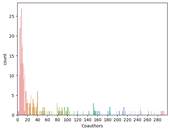
We can see the synthesized population tends to have significantly higher number of coauthors on every quartile.
The following is the distribution of the \(S_{average}\) values of the sample population.
| count | 400.000000 |
| mean | 0.749619 |
| std | 0.245596 |
| min | 0.000000 |
| 25% | 0.666667 |
| 50% | 0.800000 |
| 75% | 0.950595 |
| max | 1.000000 |
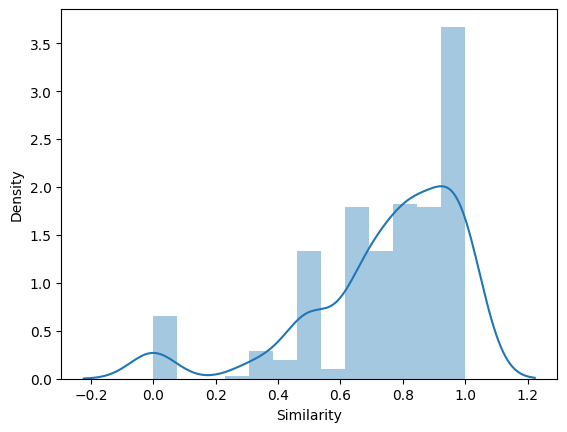
The following is the distribution of the \(S_{average}\) values of the synthesized population.
| count | 400.000000 |
| mean | 0.621903 |
| std | 0.246372 |
| min | 0.000000 |
| 25% | 0.407685 |
| 50% | 0.543210 |
| 75% | 0.870161 |
| max | 0.995765 |
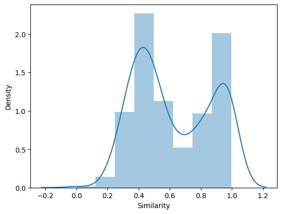
We can see that the synthesized population which consists of vertices composite of multiple authors’ representations tend to have lower similarity score with their coauthors. But what we want to know is if the difference in the two populations (sampled and synthesized) are significant enough for us to be able to train an accurate enough classifier to differentiate whether an author’s entry in the record is representative of only a single person or two different people.
Model Training
We’re using scikit-learn for the modelling, specifically its implementation of the Gaussian Naive Bayes classifier.
The following is the code snippet I use to train and test the Gaussian Naive Bayes classifier on JupyterLab.
from sklearn.model_selection import train_test_split
from sklearn.naive_bayes import GaussianNB

train, test = train_test_split(preprocessed_df, test_size=0.2)

X = train.get(['Coauthors', 'Similarity']).values
Y = train.get('Composite').astype(int).values

clf = GaussianNB()
clf.fit(X, Y)

Xt = test.get(['Coauthors', 'Similarity']).values
Yt = test.get('Composite').astype(int).values

test_predictions = clf.predict(Xt)

test_hit = 0
test_miss = 0
test_size = len(Yt)

for i in range(0, test_size):
    if test_predictions[i] == Yt[i]:
        test_hit = test_hit + 1
    else:
        test_miss = test_miss + 1
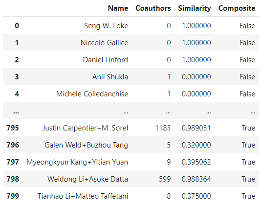
preprocessed_df is the data frame containing the whole sampled and synthesized data, along with the information such as the number of coauthors they have and the average similarity score \(S_{average}\) of the coauthors. The Composite column is the classification label, which contains the info whether the data record is originally from the sample population (which is assumed to be the representation of only one author) or the synthesized population (which is assumed to be the representation of multiple authors). The information contained in the data frame can be seen below.
I executed the training sequence 100 times with the following snippet.
training_test_repeat = 100
model_accuracy_per_epoch = []

for i in range(0, training_test_repeat):
    train, test = train_test_split(preprocessed_df, test_size=0.2)

    X = train.get(['Coauthors', 'Similarity']).values
    Y = train.get('Composite').astype(int).values

    clf = GaussianNB()
    clf.fit(X, Y)

    Xt = test.get(['Coauthors', 'Similarity']).values
    Yt = test.get('Composite').astype(int).values

    test_predictions = clf.predict(Xt)

    test_hit = 0
    test_miss = 0
    test_size = len(Yt)

    for i in range(0, test_size):
        if test_predictions[i] == Yt[i]:
            test_hit = test_hit + 1
        else:
            test_miss = test_miss + 1

    accuracy = test_hit/test_size
    model_accuracy_per_epoch.append(accuracy)
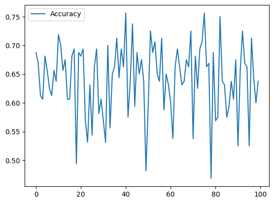
The following is the plot of the accuracy per trained model.
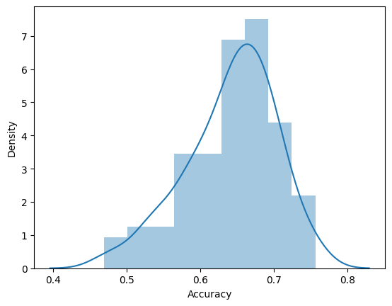
The following is the distribution of the model accuracy.
| count | 100.000000 |
| mean | 0.641312 |
| std | 0.061256 |
| min | 0.468750 |
| 25% | 0.606250 |
| 50% | 0.650000 |
| 75% | 0.687500 |
| max | 0.756250 |
I calculated the \(p\) value using this t-test calculator to calculate the statistical significance of the distribution of the model accuracy data if compared to random guessess.
We’re assuming two groups:
- Group One (\(h_0\)): \(m = 0.5\), \(s = 0.25\), \(N = 100\)
- Group Two (\(h_1\)): \(m = 0.641312\), \(s = 0.061256\), \(N = 100\)
The screenshot of the calculator’s result is as follows.
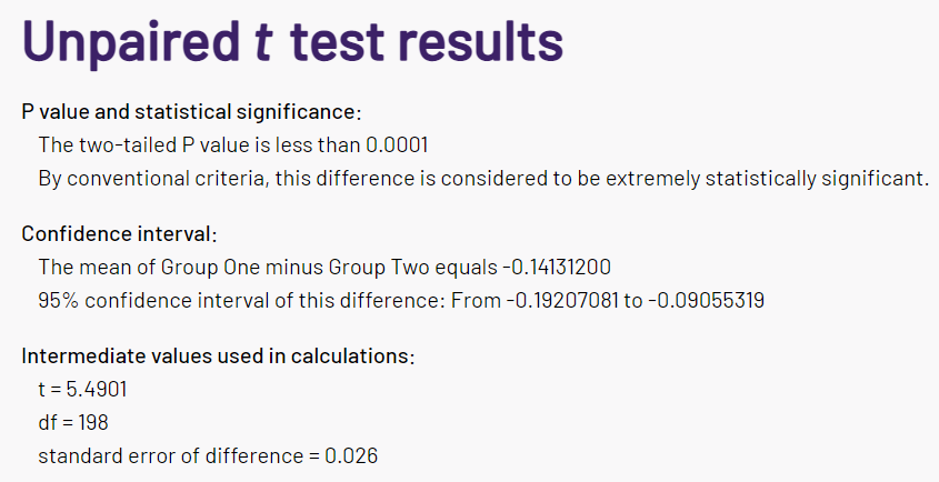
Based on the result we can say that the models’ predictions are pretty unlikely to be the result of random chance, and we can conclude that the features we used in the experiments are quite significant in recognizing whether the data comes from the sample population or the synthesized population.
Conclusion
Given the experiment results, it’s reasonable for us to conclude that it is possible differentiate between the data from sample population, which we assume to represent only one person per entry, and the data from the synthesized population, which is the combined representation of two random members of the sample population, simply by relying on the number of coauthors the author \(a\) have and the average coauthor similarities \(S_{average}\) between the author \(a\) and their coauthors \(c \in C\).
While the accuracy of the trained models mostly stays around 65% and tops around 75%, we can say that both features we used in the experiments are quite promising as they generally results in Gaussian Naive Bayes classifier models that perform well above the expected 50% accuracy for random guesses.
One noticeable weakness of this experiment is that we can’t guarantee the data we’re assuming to represent only a single author really represents only a single author. This is because we doesn’t have any references we can use as the ground truth during the experiment, and we’re simply assuming that every author entry in the original arXiv dataset represents only one person. This is unlikely to be the case, especially where the names are shortened, as multiple different people can have the same name representation in the dataset.
References
scikit-learn: machine learning in Python